Convolutional Neural Networks have changed the way we classify images. It is being used in almost all the computer vision tasks. From 2012, CNN’s have ruled the Imagenet competition, dropping the classification error rate each year. MNIST is the most studied dataset (link).

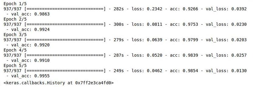
The state of the art result for MNIST dataset has an accuracy of 99.79%. In this article, we will achieve an accuracy of 99.55%.

What is the MNIST dataset?

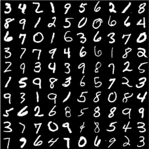
MNIST dataset contains images of handwritten digits. It has 60,000 grayscale images under the training set and 10,000 grayscale images under the test set. We will use the Keras library with Tensorflow backend to classify the images.

What is a Convolutional Neural Network?

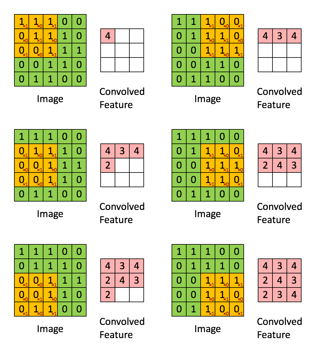
A convolution in CNN is nothing but a element wise multiplication i.e. dot product of the image matrix and the filter.

In the above example, the image is a 5 x 5 matrix and the filter going over it is a 3 x 3 matrix. A convolution operation takes place between the image and the filter and the convolved feature is generated. Each filter in a CNN, learns different characteristic of an image.

Installing Keras

Keras is a high-level neural network API, written in Python which runs on top of either Tensorflow or Theano. You can install Keras from here.

Tensorflow was developed by the Google Brain team. To learn more about it, visit there official website.

Keras was written to simplify the construction of neural nets, as tensorflow’s API is very verbose. Keras makes everything very easy and you will see it in action below. If you want to explore the tensorflow implementation of the MNIST dataset, you can find it here.

Implementation

First, we import all the necessary libraries required.

import numpy as np
import pandas as pd
import matplotlib.pyplot as plt
%matplotlib inline
from keras.datasets import mnist
from keras.models import Sequential
from keras.layers import Dense, Dropout, Activation, Flatten
from keras.optimizers import Adam
from keras.layers.normalization import BatchNormalization
from keras.utils import np_utils
from keras.layers import Conv2D, MaxPooling2D, ZeroPadding2D, GlobalAveragePooling2D
from keras.layers.advanced_activations import LeakyReLU 
from keras.preprocessing.image import ImageDataGenerator

The MNIST dataset is provided by Keras.

(X_train, y_train), (X_test, y_test) = mnist.load_data()

The shape of X_train is (60000, 28, 28). Each image has 28 x 28 resolution. The shape of X_test is (10000, 28, 28).

The input shape that a CNN accepts should be in a specific format. If you are using Tensorflow, the format should be (batch, height, width, channels). If you are using Theano, the format should be (batch, channels, height, width).

So, let’s reshape our input.

X_train = X_train.reshape(X_train.shape[0], 28, 28, 1)
X_test = X_test.reshape(X_test.shape[0], 28, 28, 1)

X_train = X_train.astype('float32')
X_test = X_test.astype('float32')

X_train/=255
X_test/=255

Now the shape of X_train is (60000, 28, 28, 1). As all the images are in grayscale, the number of channels is 1. If it was a color image, then the number of channels would be 3 (R, G, B).

Here we’ve rescaled the image data so that each pixel lies in the interval [0, 1] instead of [0, 255]. It is always a good idea to normalize the input so that each dimension has approximately the same scale.

Now, we need to one-hot encode the labels i.e. Y_train and Y_test. In one-hot encoding an integer is converted to an array which contains only one ‘1’ and the rest elements are ‘0’.

number_of_classes = 10

Y_train = np_utils.to_categorical(y_train, number_of_classes)
Y_test = np_utils.to_categorical(y_test, number_of_classes)

Y_train[0] = [0., 0., 0., 0., 0., 1., 0., 0., 0., 0.] since the label representated by it is 5.

Let’s create the model that will classify the images (the most interesting part!!).

# Three steps to create a CNN
# 1. Convolution
# 2. Activation
# 3. Pooling
# Repeat Steps 1,2,3 for adding more hidden layers

# 4. After that make a fully connected network
# This fully connected network gives ability to the CNN
# to classify the samples

model = Sequential()

model.add(Conv2D(32, (3, 3), input_shape=(28,28,1)))
model.add(BatchNormalization(axis=-1))
model.add(Activation('relu'))
model.add(Conv2D(32, (3, 3)))
model.add(BatchNormalization(axis=-1))
model.add(Activation('relu'))
model.add(MaxPooling2D(pool_size=(2,2)))

model.add(Conv2D(64,(3, 3)))
model.add(BatchNormalization(axis=-1))
model.add(Activation('relu'))
model.add(Conv2D(64, (3, 3)))
model.add(BatchNormalization(axis=-1))
model.add(Activation('relu'))
model.add(MaxPooling2D(pool_size=(2,2)))

model.add(Flatten())

# Fully connected layer
model.add(Dense(512))
model.add(BatchNormalization())
model.add(Activation('relu'))
model.add(Dropout(0.2))
model.add(Dense(10))

model.add(Activation('softmax'))

Keras allows us to specify the number of filters we want and the size of the filters. So, in our first layer, 32 is number of filters and (3, 3) is the size of the filter. We also need to specify the shape of the input which is (28, 28, 1), but we have to specify it only once.

The second layer is the Activation layer. We have used ReLU (rectified linear unit) as our activation function. ReLU function is f(x) = max(0, x), where x is the input. It sets all negative values in the matrix ‘x’ to 0 and keeps all the other values constant. It is the most used activation function since it reduces training time and prevents the problem of vanishing gradients.

The third layer is the MaxPooling layer. MaxPooling layer is used to down-sample the input to enable the model to make assumptions about the features so as to reduce over-fitting. It also reduces the number of parameters to learn, reducing the training time.

It’s a best practice to always do BatchNormalization. BatchNormalization normalizes the matrix after it is been through a convolution layer so that the scale of each dimension remains the same. It reduces the training time significantly.

After creating all the convolutional layers, we need to flatten them, so that they can act as an input to the Dense layers.

Dense layers are keras’s alias for Fully connected layers. These layers give the ability to classify the features learned by the CNN.

Dropout is the method used to reduce overfitting. It forces the model to learn multiple independent representations of the same data by randomly disabling neurons in the learning phase. In our model, dropout will randomnly disable 20% of the neurons.

The second last layer is the Dense layer with 10 neurons. The neurons in this layer should be equal to the number of classes we want to predict as this is the output layer.

The last layer is the Softmax Activation layer. Softmax activation enables us to calculate the output based on the probabilities. Each class is assigned a probability and the class with the maximum probability is the model’s output for the input.

Now we need to compile the model.

model.compile(loss='categorical_crossentropy', optimizer=Adam(), metrics=['accuracy'])

The cross-entropy loss calculates the error rate between the predicted value and the original value. The formula for calculating cross-entropy loss is given here. Categorical is used because there are 10 classes to predict from. If there were 2 classes, we would have used binary_crossentropy.

The Adam optimizer is an improvement over SGD(Stochastic Gradient Descent). The optimizer is responsible for updating the weights of the neurons via backpropagation. It calculates the derivative of the loss function with respect to each weight and subtracts it from the weight. This is how a neural network learns.

To reduce over-fitting, we use another technique known as Data Augmentation. Data augmentation rotates, shears, zooms, etc the image so that the model learns to generalize and not remember specific data. If the model overfits, it will perform very well on the images that it already knows but will fail if new images are given to it.

gen = ImageDataGenerator(rotation_range=8, width_shift_range=0.08, shear_range=0.3,
                         height_shift_range=0.08, zoom_range=0.08)

test_gen = ImageDataGenerator()

This is how we can do Data Augmentation in Keras. You can play with the values and check if it improves the accuracy of the model.

We have to create batches, so that we use less memory. Moreover, we can also train our model faster by creating batches. Here we are using batch of 64, so the model will take 64 images at a time and train on them.

train_generator = gen.flow(X_train, Y_train, batch_size=64)
test_generator = test_gen.flow(X_test, Y_test, batch_size=64)

It’s Training Time!!

model.fit_generator(train_generator, steps_per_epoch=60000//64, epochs=5, 
                    validation_data=test_generator, validation_steps=10000//64)

We achived 99.55% accuracy using this simple model. To improve the result, we can do ensembling of models. We can also use pseudo labelling to improve the accuracy.

Visualization of Convolutional Layers

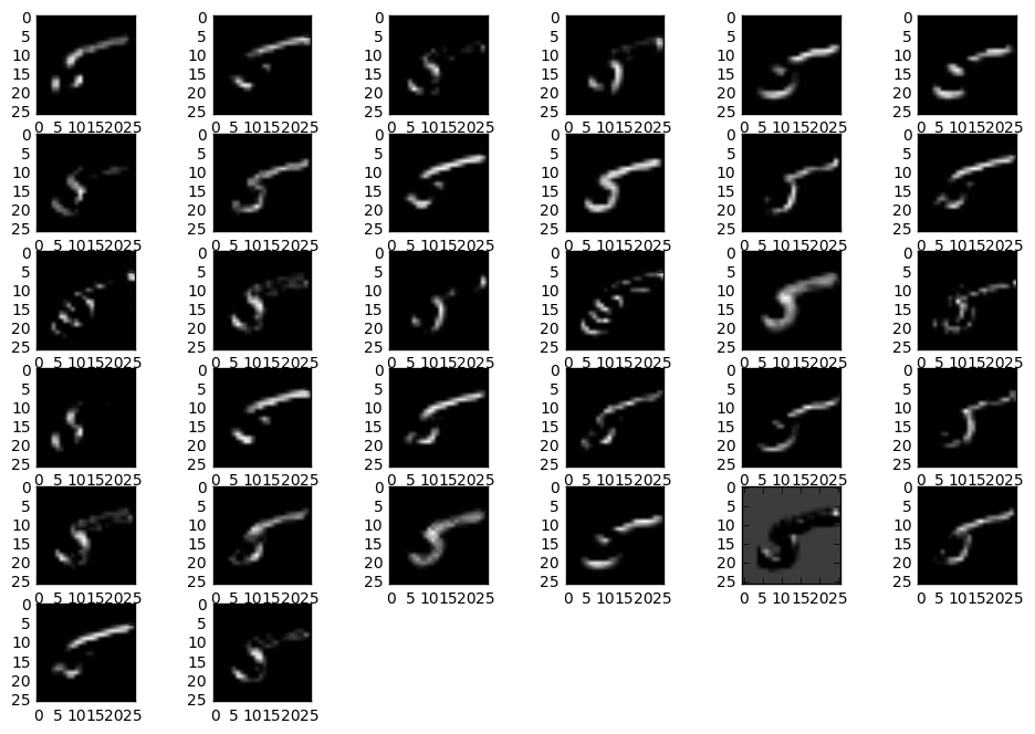
This is what a CNN learns. As you can see, some filters have learnt to recognize edges, curves, etc. This is the output of the first ReLU activation layer.

You can find the entire code here.

The code for visualization of Convolutional Layers can be found here. I have used Theano as a backend for this code.

This is an awesome neural network 3D simulation video based on the MNIST dataset.

If you’re interested in collaborating, discussing or working with me on an exciting idea, contact me at yash DOT katariya10 AT gmail.com

Until next time,

Ciao

Tweet